Training on ST-MNIST with Tonic + snnTorch Tutorial
Tutorial written by Dylan Louie (djlouie@ucsc.edu), Hannah Cohen Sandler (hcohensa@ucsc.edu), Shatoparba Banerjee (sbaner12@ucsc.edu)
The snnTorch tutorial series is based on the following paper. If you find these resources or code useful in your work, please consider citing the following source:
Note
- This tutorial is a static non-editable version. Interactive, editable versions are available via the following links:
pip install tonic
pip install snntorch
# tonic imports
import tonic
import tonic.transforms as transforms  # Not to be mistaken with torchdata.transfroms
from tonic import DiskCachedDataset

# torch imports
import torch
from torch.utils.data import random_split
from torch.utils.data import DataLoader
import torchvision
import torch.nn as nn

# snntorch imports
import snntorch as snn
from snntorch import surrogate
import snntorch.spikeplot as splt
from snntorch import functional as SF
from snntorch import utils

# other imports
import matplotlib.pyplot as plt
from IPython.display import HTML
from IPython.display import display
import numpy as np
import torchdata
import os
from ipywidgets import IntProgress
import time
import statistics
1. The ST-MNIST Dataset
1.1 Introduction
The Spiking Tactile-MNIST (ST-MNIST) dataset features handwritten digits (0-9) inscribed by 23 individuals on a 100-taxel biomimetic event-based tactile sensor array. This dataset captures the dynamic pressure changes associated with natural writing. The tactile sensing system, Asynchronously Coded Electronic Skin (ACES), emulates the human peripheral nervous system, transmitting fast-adapting (FA) responses as asynchronous electrical events.
More information about the ST-MNIST dataset can be found in the following paper:
1.2 Downloading the ST-MNIST dataset
ST-MNIST is in the MAT format. Tonic can be used transform this into
an event-based format (x, y, t, p).
Download the compressed dataset by accessing: https://scholarbank.nus.edu.sg/bitstream/10635/168106/2/STMNIST%20dataset%20NUS%20Tee%20Research%20Group.zip
The zip file is
STMNIST dataset NUS Tee Research Group. Create a parent folder titledSTMNISTand place the zip file inside.If running in a cloud-based environment, e.g., on Colab, you will need to do this in Google Drive.
1.3 Mount to Drive
You may need to authorize the following to access Google Drive:
# Load the Drive helper and mount
from google.colab import drive
drive.mount('/content/drive')
After executing the cell above, Drive files will be present in
“/content/drive/MyDrive”. You may need to change the root file to
your own path.
root = "/content/drive/My Drive/"  # similar to os.path.join('content', 'drive', 'My Drive')
os.listdir(os.path.join(root, 'STMNIST')) # confirm the file exists
1.4 ST-MNIST Using Tonic
Tonic will be used to convert the dataset into a format compatible
with PyTorch/snnTorch. The documentation can be found
here.
dataset = tonic.prototype.datasets.STMNIST(root=root, keep_compressed = False, shuffle = False)
Tonic formats the STMNIST dataset into (x, y, t, p) tuples.
xis the position on the x-axisyis the position on the y-axistis a timestamppis polarity; +1 if taxel pressed down, 0 if taxel released
Each sample also contains the label, which is an integer 0-9 that corresponds to what digit is being drawn.
An example of one of the events is shown below:
events, target = next(iter(dataset))
print(events[0])
print(target)
>>> (2, 7, 199838, 0)
>>> 6
The .ToFrame() function from tonic.transforms transforms events
from an (x, y, t, p) tuple to a numpy array matrix.
sensor_size = tuple(tonic.prototype.datasets.STMNIST.sensor_size.values())  # The sensor size for STMNIST is (10, 10, 2)

# filter noisy pixels and integrate events into 1ms frames
frame_transform = transforms.Compose([transforms.Denoise(filter_time=10000),
                                      transforms.ToFrame(sensor_size=sensor_size,
                                                         time_window=20000)
                                     ])

transformed_events = frame_transform(events)

print_frame(transformed_events)
>>>
----------------------------
[[[0 0 0 0 0 0 0 0 0 0]
[0 0 0 0 0 0 0 0 0 0]
[0 0 0 0 0 0 0 0 0 0]
[0 0 0 0 0 0 0 0 0 0]
[0 0 0 0 0 0 0 0 0 0]
[0 0 0 0 0 0 0 0 0 0]
[0 3 4 0 0 0 0 0 0 0]
[0 2 0 0 0 0 0 0 0 0]
[0 0 0 0 0 0 0 0 0 0]
[0 0 0 0 0 0 0 0 0 0]]

[[0 0 0 0 0 0 0 0 0 0]
[0 0 0 0 0 0 0 0 0 0]
[0 0 0 0 0 0 0 0 0 0]
[0 0 0 0 0 0 0 0 0 0]
[0 0 0 0 0 0 0 0 0 0]
[0 0 4 0 0 0 0 0 0 0]
[0 6 3 0 0 0 0 0 0 0]
[0 0 0 0 0 0 0 0 0 0]
[0 0 0 0 0 0 0 0 0 0]
[0 0 0 0 0 0 0 0 0 0]]]
----------------------------
[[0 0 0 0 0 0 0 0 0 0]
[0 0 0 0 0 0 0 0 0 0]
[0 0 0 0 0 0 0 0 0 0]
[0 0 0 0 0 0 0 0 0 0]
[0 0 0 0 0 0 0 0 0 0]
[0 0 0 0 0 0 0 0 0 0]
[0 3 4 0 0 0 0 0 0 0]
[0 2 0 0 0 0 0 0 0 0]
[0 0 0 0 0 0 0 0 0 0]
[0 0 0 0 0 0 0 0 0 0]]
----------------------------
[0 0 0 0 0 0 0 0 0 0]
1.5 Visualizations
Using tonic.utils.plot_animation, the frame transform, and also some
rotation. We can create an animation of the data and visualize this.
# Iterate to a new iteration
events, target = next(iter(dataset))
frame_transform_tonic_visual = tonic.transforms.ToFrame(
    sensor_size=(10, 10, 2),
    time_window=10000,
)

frames = frame_transform_tonic_visual(events)
frames = frames / np.max(frames)
frames = np.rot90(frames, k=-1, axes=(2, 3))
frames = np.flip(frames, axis=3)

# Print out the Target
print('Animation of ST-MNIST')
print('The target label is:',target)
animation = tonic.utils.plot_animation(frames)

# Display the animation inline in a Jupyter notebook
HTML(animation.to_jshtml())
We can also use snntorch.spikeplot
frame_transform_snntorch_visual = tonic.transforms.ToFrame(
    sensor_size=(10, 10, 2),
    time_window=8000,
)

tran = frame_transform_snntorch_visual(events)
tran = np.rot90(tran, k=-1, axes=(2, 3))
tran = np.flip(tran, axis=3)
tran = torch.from_numpy(tran)

tensor1 = tran[:, 0:1, :, :]
tensor2 = tran[:, 1:2, :, :]

print('Animation of ST-MNIST')
print('The target label is:',target)

fig, ax = plt.subplots()
time_steps = tensor1.size(0)
tensor1_plot = tensor1.reshape(time_steps, 10, 10)
anim = splt.animator(tensor1_plot, fig, ax, interval=10)

display(HTML(anim.to_html5_video()))
>>> Animation of ST-MNIST
>>> The target label is: 3
There is a total of 6,953 recordings in this dataset. The developers of ST-MNIST invited 23 participants to write each 10 digit approx. 30 times each: 23*30*10 = 6,900.
print(len(dataset))
>>> 6953
1.6 Lets create a trainset and testset!
ST-MNIST isn’t already seperated into a trainset and testset in Tonic.
That means we will have to seperate it manually. In the process of
seperating the data we will transform them using .ToFrame() as well.
sensor_size = tonic.prototype.datasets.STMNIST.sensor_size
sensor_size = tuple(sensor_size.values())

# Define a transform
frame_transform = transforms.Compose([transforms.ToFrame(sensor_size=sensor_size, time_window=20000)])
The following code reads out the a portion of the dataset, transforms
the events using frame_transform defined above, and then seperates
the data into a trainset and a testset. On top of that, .ToFrame()
is applied each time. Thus, this code snippet might take a few minutes.
For speed, we will just use a subset of the dataset. By default, 640 training samples and 320 testing samples. Feel free to change this if you have more patience than us.
def shorter_transform_STMNIST(data, transform):
    short_train_size = 640
    short_test_size = 320

    train_bar = IntProgress(min=0, max=short_train_size)
    test_bar = IntProgress(min=0, max=short_test_size)

    testset = []
    trainset = []

    print('Porting over and transforming the trainset.')
    display(train_bar)
    for _ in range(short_train_size):
        events, target = next(iter(dataset))
        events = transform(events)
        trainset.append((events, target))
        train_bar.value += 1
    print('Porting over and transforming the testset.')
    display(test_bar)
    for _ in range(short_test_size):
        events, target = next(iter(dataset))
        events = transform(events)
        testset.append((events, target))
        test_bar.value += 1

    return (trainset, testset)

start_time = time.time()
trainset, testset = shorter_transform_STMNIST(dataset, frame_transform)
elapsed_time = time.time() - start_time

# Convert elapsed time to minutes, seconds, and milliseconds
minutes, seconds = divmod(elapsed_time, 60)
seconds, milliseconds = divmod(seconds, 1)
milliseconds = round(milliseconds * 1000)

# Print the elapsed time
print(f"Elapsed time: {int(minutes)} minutes, {int(seconds)} seconds, {milliseconds} milliseconds")
1.6 Dataloading and Batching
# Create a DataLoader
dataloader = DataLoader(trainset, batch_size=32, shuffle=True)
For faster dataloading, we can use DiskCashedDataset(...) from
Tonic.
Due to variations in the lengths of event recordings,
tonic.collation.PadTensors() will be used to prevent irregular
tensor shapes. Shorter recordings are padded, ensuring uniform
dimensions across all samples in a batch.
transform = tonic.transforms.Compose([torch.from_numpy])

cached_trainset = DiskCachedDataset(trainset, transform=transform, cache_path='./cache/stmnist/train')

# no augmentations for the testset
cached_testset = DiskCachedDataset(testset, cache_path='./cache/stmnist/test')

batch_size = 32
trainloader = DataLoader(cached_trainset, batch_size=batch_size, collate_fn=tonic.collation.PadTensors(batch_first=False), shuffle=True)
testloader = DataLoader(cached_testset, batch_size=batch_size, collate_fn=tonic.collation.PadTensors(batch_first=False))
# Query the shape of a sample: time x batch x dimensions
data_tensor, targets = next(iter(trainloader))
print(data_tensor.shape)
>>> torch.Size([89, 32, 2, 10, 10])
1.7 Create the Spiking Convolutional Neural Network
Below we have by default a spiking convolutional neural network with the
architecture: 10×10-32c4-64c3-MaxPool2d(2)-10o.
device = torch.device("cuda") if torch.cuda.is_available() else torch.device("cpu")

# neuron and simulation parameters
beta = 0.95

# This is the same architecture that was used in the STMNIST Paper
scnn_net = nn.Sequential(
    nn.Conv2d(2, 32, kernel_size=4),
    snn.Leaky(beta=beta, init_hidden=True),
    nn.Conv2d(32, 64, kernel_size=3),
    snn.Leaky(beta=beta, init_hidden=True),
    nn.MaxPool2d(2),
    nn.Flatten(),
    nn.Linear(64 * 2 * 2, 10),  # Increased size of the linear layer
    snn.Leaky(beta=beta, init_hidden=True, output=True)
).to(device)

optimizer = torch.optim.Adam(scnn_net.parameters(), lr=2e-2, betas=(0.9, 0.999))
loss_fn = SF.mse_count_loss(correct_rate=0.8, incorrect_rate=0.2)
1.8 Define the Forward Pass
def forward_pass(net, data):
    spk_rec = []
    utils.reset(net)  # resets hidden states for all LIF neurons in net

    for step in range(data.size(0)):  # data.size(0) = number of time steps

        spk_out, mem_out = net(data[step])
        spk_rec.append(spk_out)

    return torch.stack(spk_rec)
1.9 Create and Run the Training Loop
This might take a while, so kick back, take a break and eat a snack while this happens; perhaps even count kangaroos to take a nap or do a shoey and get schwasted instead.
start_time = time.time()

num_epochs = 30

loss_hist = []
acc_hist = []

# training loop
for epoch in range(num_epochs):
    for i, (data, targets) in enumerate(iter(trainloader)):
        data = data.to(device)
        targets = targets.to(device)

        scnn_net.train()
        spk_rec = forward_pass(scnn_net, data)
        loss_val = loss_fn(spk_rec, targets)

        # Gradient calculation + weight update
        optimizer.zero_grad()
        loss_val.backward()
        optimizer.step()

        # Store loss history for future plotting
        loss_hist.append(loss_val.item())

        # Print loss every 4 iterations
        if i%4 == 0:
            print(f"Epoch {epoch}, Iteration {i} \nTrain Loss: {loss_val.item():.2f}")

        # Calculate accuracy rate and then append it to accuracy history
        acc = SF.accuracy_rate(spk_rec, targets)
        acc_hist.append(acc)

        # Print accuracy every 4 iterations
        if i%4 == 0:
            print(f"Accuracy: {acc * 100:.2f}%\n")

end_time = time.time()

# Calculate elapsed time
elapsed_time = end_time - start_time

# Convert elapsed time to minutes, seconds, and milliseconds
minutes, seconds = divmod(elapsed_time, 60)
seconds, milliseconds = divmod(seconds, 1)
milliseconds = round(milliseconds * 1000)

# Print the elapsed time
print(f"Elapsed time: {int(minutes)} minutes, {int(seconds)} seconds, {milliseconds} milliseconds")
Epoch 0, Iteration 0
Train Loss: 8.06
Accuracy: 9.38%

Epoch 0, Iteration 4
Train Loss: 42.37
Accuracy: 6.25%

Epoch 0, Iteration 8
Train Loss: 7.07
Accuracy: 15.62%

Epoch 0, Iteration 12
Train Loss: 8.73
Accuracy: 12.50%

...

Epoch 29, Iteration 8
Train Loss: 0.93
Accuracy: 100.00%

Epoch 29, Iteration 12
Train Loss: 0.97
Accuracy: 100.00%

Epoch 29, Iteration 16
Train Loss: 1.38
Accuracy: 87.50%

Elapsed time: 2 minutes, 45 seconds, 187 milliseconds
Uncomment the code below if you want to save the model
# torch.save(scnn_net.state_dict(), 'scnn_net.pth')
2. Results
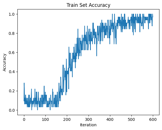
2.1 Plot accuracy history
# Plot Loss
fig = plt.figure(facecolor="w")
plt.plot(acc_hist)
plt.title("Train Set Accuracy")
plt.xlabel("Iteration")
plt.ylabel("Accuracy")
plt.show()
2.2 Evaluate the Network on the Test Set
# Make sure your model is in evaluation mode
scnn_net.eval()

# Initialize variables to store predictions and ground truth labels
acc_hist = []

# Iterate over batches in the testloader
with torch.no_grad():
    for data, targets in testloader:
        # Move data and targets to the device (GPU or CPU)
        data = data.to(device)
        targets = targets.to(device)

        # Forward pass
        spk_rec = forward_pass(scnn_net, data)

        acc = SF.accuracy_rate(spk_rec, targets)
        acc_hist.append(acc)

        # if i%10 == 0:
        # print(f"Accuracy: {acc * 100:.2f}%\n")

print("The average loss across the testloader is:", statistics.mean(acc_hist))
>>> The average loss across the testloader is: 0.65
2.3 Visualize Spike Recordings
The following visual is a spike count histogram for a single target and single piece of data using the spike recording list.
spk_rec = forward_pass(scnn_net, data)
# Change index to visualize a different sample
idx = 0
fig, ax = plt.subplots(facecolor='w', figsize=(12, 7))
labels=['0', '1', '2', '3', '4', '5', '6', '7', '8','9']
print(f"The target label is: {targets[idx]}")

#  Plot spike count histogram
anim = splt.spike_count(spk_rec[:, idx].detach().cpu(), fig, ax, labels=labels,
                        animate=True, interpolate=1)

display(HTML(anim.to_html5_video()))
# anim.save("spike_bar.mp4")
Congratulations!
You trained a Spiking CNN using snnTorch and Tonic on ST-MNIST!