教程(五) - 使用snnTorch训练脉冲神经网络
本教程出自 Jason K. Eshraghian (www.ncg.ucsc.edu)
snnTorch 教程系列基于以下论文。如果您发现这些资源或代码对您的工作有用,请考虑引用以下来源:
Note
- 本教程是不可编辑的静态版本。交互式可编辑版本可通过以下链接获取:
简介
在本教程中,你将:
了解脉冲神经元如何作为递归网络实现
通过时间了解反向传播,以及 SNN 中的相关挑战,如脉冲的不可微分性
在静态 MNIST 数据集上训练全连接网络
本教程的部分灵感来自 Friedemann Zenke 在 SNN 方面的大量工作。 请在 这里 查看他关于替代梯度的资料库, 以及我最喜欢的一篇论文: E. O. Neftci, H. Mostafa, F. Zenke,
SNN中的替代梯度学习: 将基于梯度的优化功能引入SNN。 IEEE Signal Processing Magazine 36, 51-63.
在教程的最后,我们将实施一种基本的监督学习算法。 我们将使用原始静态 MNIST 数据集,并使用梯度下降法训练 多层 全连接 脉冲神经网络 来执行图像分类。
安装 snnTorch 的最新 PyPi 发行版:
$ pip install snntorch
# imports
import snntorch as snn
from snntorch import spikeplot as splt
from snntorch import spikegen

import torch
import torch.nn as nn
from torch.utils.data import DataLoader
from torchvision import datasets, transforms

import matplotlib.pyplot as plt
import numpy as np
import itertools
1. 脉冲神经网络的递归表示
在 教程(三) 中, 我们推导出了泄漏整合-发射(LIF)神经元的递归表示:
其中,输入突触电流解释为 \(I_{\rm in}[t] = WX[t]\), 而 \(X[t]\) 可以是任意输入的脉冲、 阶跃/时变电压或非加权阶跃/时变电流。 脉冲用下式表示,如果膜电位超过阈值,就会发出一个脉冲:
这种离散递归形式的脉冲神经元表述几乎可以完美利用训练递归神经网络(RNN) 和基于序列模型的发展。我们使用一个*隐式*递归连接来说明膜电位的衰减, 并将其与*显式*递归区分开来,在*显式*递归中, 输出脉冲 \(S_{\rm out}`被反馈回输入。 在下图中, 权重为 :math:`U_{\rm thr}`的连接代表着复位机制:math:`R[t]\)。
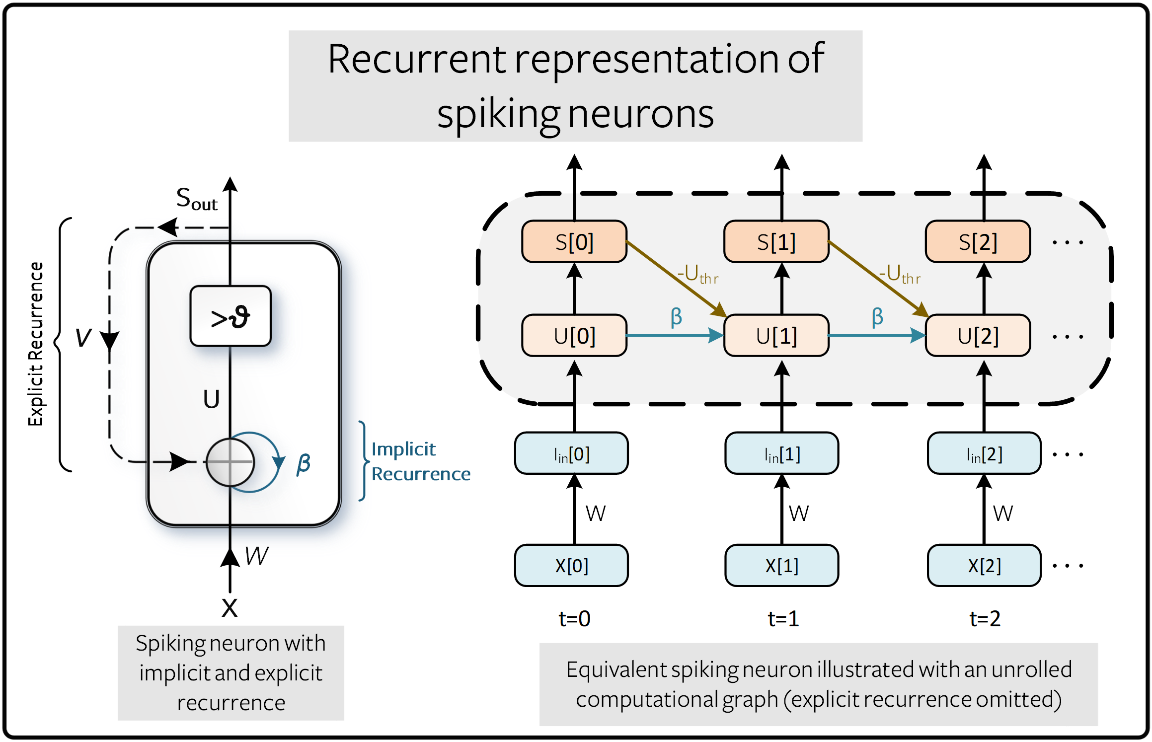
展开图的好处在于,它明确描述了计算是如何进行的。 展开过程说明了信息流在时间上的前向(从左到右),以计算输出和损失, 以及在时间上的后向,以计算梯度。模拟的时间步数越多,图形就越深。
传统的 RNN 将 \(\beta\) 视为可学习的参数。 这对 SNN 也是可行的, 不过默认情况下, 它们被视为超参数(hyperparameters)。 这就用超参数搜索取代了梯度消失和梯度爆炸问题。 未来的教程将介绍如何使 \(\beta\) 成为可学习参数。
2. 脉冲的不可微分性
2.1 使用反向传播算法进行训练
表示 \(S\) 和 \(U\) 之间关系的另一种方法是:
其中 \(\Theta(\cdot)\) 是 Heaviside 阶跃函数(其实就是在原点发生阶跃的函数):

以这种形式训练网络会带来一些严峻的挑战。 考虑上图中题为 “脉冲神经元的递归表示” 的计算图的一个单独的时间步, 如下图 前向传递 所示:
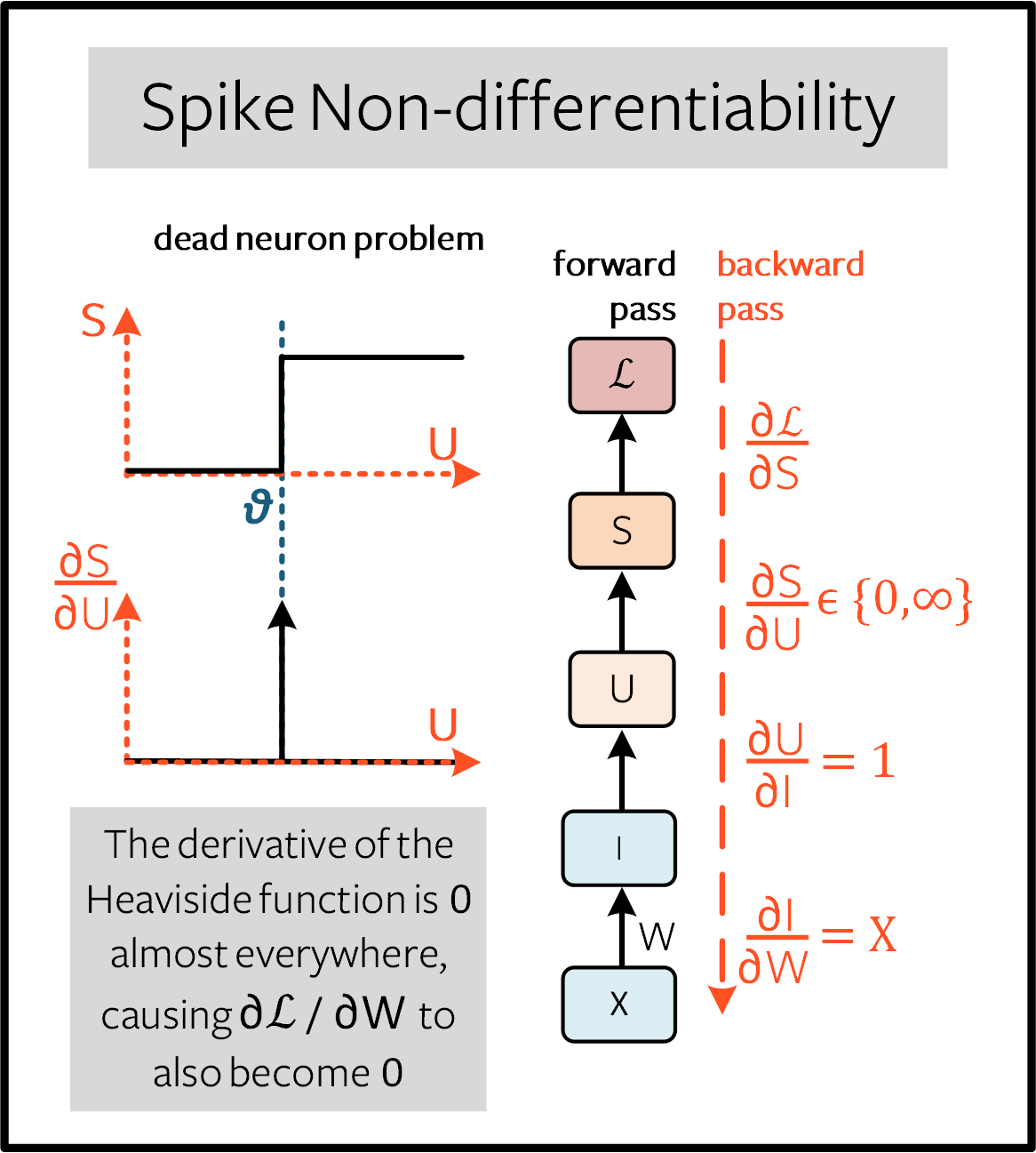
我们的目标是利用损失相对于权重的梯度来训练网络,从而更新权重,使损失最小化。 反向传播算法利用链式规则实现了这一目标:
从 \((1)\), \(/partial I//partial W=X\), 以及 \(partial U//partial I=1\)。 虽然没定义损失函数, 我们还是可以假设 \(\partial \mathcal{L}/\partial S\) 有一个解析解,有一个类似于交叉熵或均方误差损失(稍后会详细介绍)的解析解。
我们真正要处理的项是 \(\partial S/\partial U\)。 (3)中的Heaviside阶跃函数的导数是狄拉克-德尔塔函数, 它在任何地方都求值为 \(0\), 但在阈值处除外 \(U_{\rm thr} = \theta\), 在这里它趋于无穷大。这意味着 梯度几乎总是归零 (如果 \(U\) 恰好位于阈值处,则为饱和而不是归零), 无法进行学习。这被称为 死神经元问题 。
2.2 克服死神经元问题
解决死神经元问题的最常见方法是在前向传递过程中保持Heaviside函数的原样, 但将导数项 \(\partial S/\partial U\) 换成在后向传递过程中不会扼杀学习过程的导数项, 即 \(\partial \tilde{S}/\partial U\)。这听起来可能有些奇怪, 但事实证明,神经网络对这种近似是相当稳健的。这就是通常所说的 替代梯度 方法。
使用替代梯度有多种选择, 我们将在 教程(六)” 中详细介绍这些方法。 snnTorch 的默认方法(截至 v0.6.0)是用反正切函数平滑 Heaviside 函数。 使用的后向导数为
其中左箭头表示替换。
下面用 PyTorch 实现了 \((1)-(2)\) 中描述的同一个神经元模型 (就是教程(三)中的 snn.Leaky 神经元)。如果您不理解,请不要担心。 稍后我们将使用 snnTorch 将其浓缩为一行代码:
# Leaky neuron model, overriding the backward pass with a custom function
class LeakySurrogate(nn.Module):
  def __init__(self, beta, threshold=1.0):
      super(LeakySurrogate, self).__init__()

      # initialize decay rate beta and threshold
      self.beta = beta
      self.threshold = threshold
      self.spike_gradient = self.ATan.apply

  # the forward function is called each time we call Leaky
  def forward(self, input_, mem):
    spk = self.spike_gradient((mem-self.threshold))  # call the Heaviside function
    reset = (self.beta * spk * self.threshold).detach()  # remove reset from computational graph
    mem = self.beta * mem + input_ - reset  # Eq (1)
    return spk, mem

  # Forward pass: Heaviside function
  # Backward pass: Override Dirac Delta with the derivative of the ArcTan function
  @staticmethod
  class ATan(torch.autograd.Function):
      @staticmethod
      def forward(ctx, mem):
          spk = (mem > 0).float() # Heaviside on the forward pass: Eq(2)
          ctx.save_for_backward(mem)  # store the membrane for use in the backward pass
          return spk

      @staticmethod
      def backward(ctx, grad_output):
          (spk,) = ctx.saved_tensors  # retrieve the membrane potential
          grad = 1 / (1 + (np.pi * mem).pow_(2)) * grad_output # Eqn 5
          return grad
请注意,重置机制是与计算图分离的,因为替代梯度只应用于 \(\partial S/\partial U\) 而不是 \(\partial R/\partial U\)。
以上神经元可以这样实现:
lif1 = LeakySurrogate(beta=0.9)
这个神经元可以用 for 循环来模拟,就像之前的教程一样。 PyTorch 的自动差异化(autodiff)机制会在后台跟踪梯度。
调用 snn.Leaky 神经元也能实现同样的效果。
事实上,每次从 snnTorch 调用任何神经元模型时,
ATan 替代梯度都会默认应用于该神经元:
lif1 = snn.Leaky(beta=0.9)
如果您想了解该神经元的行为,请参阅 教程(三).
3. 通过时间反向传播(BPTT)
方程 \((4)\) 仅计算一个单一时间步的梯度(在下图中称为 即时影响), 但是通过时间反向传播(BPTT)算法计算 从损失到 所有 后代(descendants)的梯度并将它们相加。
权重 \(W\) 在每个时间步都应用,因此可以想象在每个时间步也计算了损失。 权重对当前和历史损失的影响必须相加在一起以定义全局梯度:
方程 \((5)\) 的目的是确保因果关系: 通过限制 \(s\leq t\),我们只考虑了权重 \(W\) 对损失的即时和先前影响的贡献。 循环系统将权重限制为在所有步骤中共享:\(W[0]=W[1] =~... ~ = W\)。 因此,对于所有的 \(W\),改变 \(W[s]\) 将对所有 \(W\) 产生相同的影响, 这意味着 \(\partial W[s]/\partial W=1\):
举个例子,隔离由于 \(s = t-1\) 仅 导致的先前影响; 这意味着反向传递必须回溯一步。可以将 \(W[t-1]\) 对损失的影响写成:
我们已经处理了来自方程 \((4)\) 的所有这些项, 除了 \(\partial U[t]/\partial U[t-1]\)。 根据方程 \((1)\),这个时间导数项简单地等于 \(\beta\)。 因此,如果我们真的想,我们现在已经知道足够的信息来手动(且痛苦地) 计算每个时间步的每个权重的导数,对于单个神经元,它会看起来像这样:

但幸运的是,PyTorch 的自动微分在后台为我们处理这些。
Note
以上图中省略了重置机制。在 snnTorch 中,重置包含在前向传递中,但与反向传递分离。
4. 设置损失函数 / 输出解码
在传统的非脉冲神经网络中,有监督的多类分类问题会选取 激活度最高的神经元,并将其作为预测类别。
在脉冲神经网络中,有多种解释输出脉冲的方式。最常见的方法包括:
脉冲率编码: 选择具有最高脉冲率(或脉冲计数)的神经元作为预测类别
延迟编码: 选择首先发放脉冲的神经元作为预测类别
这可能会让你联想到关于 教程(一)神经编码。不同之处在于,在这里,我们是在解释(解码)输出脉冲,而不是将原始输入数据编码/转换成脉冲。
让我们专注于脉冲率编码。当输入数据传递到网络时, 我们希望正确的神经元类别在仿真运行的过程中发射最多的脉冲。 这对应于最高的平均脉冲频率。实现这一目标的一种方法是增加正确类别的膜电位至 \(U>U_{\rm thr}\), 并将不正确类别的膜电位设置为 \(U<U_{\rm thr}\)。 将目标应用于 \(U\) 作为调节脉冲行为从 \(S\) 到 \(U\) 的代理。
这可以通过对输出神经元的膜电位取softmax来实现,其中 \(C\) 是输出类别的数量:
通过以下方式获取 \(p_i\) 和目标 \(y_i \in \{0,1\}^C\) 之间的交叉熵, 目标是一个独热(one-hot)目标向量:
实际效果是,鼓励正确类别的膜电位增加,而不正确类别的膜电位降低。 这意味着在所有时间步中鼓励正确类别激活,且在所有时间步中抑制不正确类别。 这可能不是脉冲神经网络的最高效实现之一,但它是其中最简单的之一。
这个目标应用于仿真的每个时间步,因此也在每个步骤生成一个损失。 然后在仿真结束时将这些损失相加:
这只是将损失函数应用于脉冲神经网络的众多可能方法之一。
在 snnTorch 中,有多种方法可用(在模块 snn.functional 中),
他们将成为未来教程的主题。
所有的背景理论介绍完毕,我们现在终于可以开始训练一个全连接的脉冲神经网络。
5. 配置静态MNIST数据集
# dataloader arguments
batch_size = 128
data_path='/tmp/data/mnist'

dtype = torch.float
device = torch.device("cuda") if torch.cuda.is_available() else torch.device("mps") if torch.backends.mps.is_available() else torch.device("cpu")
# Define a transform
transform = transforms.Compose([
            transforms.Resize((28, 28)),
            transforms.Grayscale(),
            transforms.ToTensor(),
            transforms.Normalize((0,), (1,))])

mnist_train = datasets.MNIST(data_path, train=True, download=True, transform=transform)
mnist_test = datasets.MNIST(data_path, train=False, download=True, transform=transform)
# Create DataLoaders
train_loader = DataLoader(mnist_train, batch_size=batch_size, shuffle=True, drop_last=True)
test_loader = DataLoader(mnist_test, batch_size=batch_size, shuffle=True, drop_last=True)
6. 定义网络
# Network Architecture
num_inputs = 28*28
num_hidden = 1000
num_outputs = 10

# Temporal Dynamics
num_steps = 25
beta = 0.95
# Define Network
class Net(nn.Module):
    def __init__(self):
        super().__init__()

        # Initialize layers
        self.fc1 = nn.Linear(num_inputs, num_hidden)
        self.lif1 = snn.Leaky(beta=beta)
        self.fc2 = nn.Linear(num_hidden, num_outputs)
        self.lif2 = snn.Leaky(beta=beta)

    def forward(self, x):

        # Initialize hidden states at t=0
        mem1 = self.lif1.init_leaky()
        mem2 = self.lif2.init_leaky()

        # Record the final layer
        spk2_rec = []
        mem2_rec = []

        for step in range(num_steps):
            cur1 = self.fc1(x)
            spk1, mem1 = self.lif1(cur1, mem1)
            cur2 = self.fc2(spk1)
            spk2, mem2 = self.lif2(cur2, mem2)
            spk2_rec.append(spk2)
            mem2_rec.append(mem2)

        return torch.stack(spk2_rec, dim=0), torch.stack(mem2_rec, dim=0)

# Load the network onto CUDA if available
net = Net().to(device)
forward() 函数中的代码将只在明确传递输入参数 x 到 net 时才被调用。
fc1对来自MNIST数据集的所有输入像素应用线性变换;lif1集成了随时间变化的加权输入,如果满足阈值条件,则发放脉冲;fc2对lif1的输出脉冲应用线性变换;lif2是另一层脉冲神经元,集成了随时间变化的加权脉冲。
7. 训练SNN
7.1 准确率指标(Accuracy Metric)
下面这个函数会获取一批数据、统计每个神经元的所有脉冲(即模拟时间内的脉冲率代码), 并将最高计数的索引与实际目标进行比较。如果两者匹配,则说明网络正确预测了目标。
# pass data into the network, sum the spikes over time
# and compare the neuron with the highest number of spikes
# with the target

def print_batch_accuracy(data, targets, train=False):
    output, _ = net(data.view(batch_size, -1))
    _, idx = output.sum(dim=0).max(1)
    acc = np.mean((targets == idx).detach().cpu().numpy())

    if train:
        print(f"Train set accuracy for a single minibatch: {acc*100:.2f}%")
    else:
        print(f"Test set accuracy for a single minibatch: {acc*100:.2f}%")

def train_printer():
    print(f"Epoch {epoch}, Iteration {iter_counter}")
    print(f"Train Set Loss: {loss_hist[counter]:.2f}")
    print(f"Test Set Loss: {test_loss_hist[counter]:.2f}")
    print_batch_accuracy(data, targets, train=True)
    print_batch_accuracy(test_data, test_targets, train=False)
    print("\n")
7.2 损失定义(Loss Definition)
PyTorch 中的 nn.CrossEntropyLoss 函数会自动处理输出层的Softmax,
并在输出处生成损失。
loss = nn.CrossEntropyLoss()
7.3 优化器(Optimizer)
Adam 是一个稳健的优化器,在递归网络中表现出色, 因此我们应用Adam并将其学习率为 \(5\times10^{-4}\)。
optimizer = torch.optim.Adam(net.parameters(), lr=5e-4, betas=(0.9, 0.999))
7.4 一次训练迭代
获取第一批数据并将其加载到CUDA(如果可以)。
data, targets = next(iter(train_loader))
data = data.to(device)
targets = targets.to(device)
将输入数据拍扁为大小为 \(784\) 的向量,并将其传入网络。
spk_rec, mem_rec = net(data.view(batch_size, -1))
>>> print(mem_rec.size())
torch.Size([25, 128, 10])
膜电位记录跨度为
25 个时间步长
128 个数据样本
10 个输出神经元
我们希望计算每个时间步长的损耗,并将这些损耗相加。 我们希望按照公式 \((10)\) 计算出每个时间步的损失,并将这些损失相加:
# initialize the total loss value
loss_val = torch.zeros((1), dtype=dtype, device=device)

# sum loss at every step
for step in range(num_steps):
  loss_val += loss(mem_rec[step], targets)
>>> print(f"Training loss: {loss_val.item():.3f}")
Training loss: 60.488
损失相当大,因为它是 25 个时间步长的总和。 准确率也很低(大约应在 10%左右),因为网络还未经训练:
>>> print_batch_accuracy(data, targets, train=True)
Train set accuracy for a single minibatch: 10.16%
对网络进行一次权重更新:
# clear previously stored gradients
optimizer.zero_grad()

# calculate the gradients
loss_val.backward()

# weight update
optimizer.step()
现在,在一次迭代后重新运行损失计算和精度:
# calculate new network outputs using the same data
spk_rec, mem_rec = net(data.view(batch_size, -1))

# initialize the total loss value
loss_val = torch.zeros((1), dtype=dtype, device=device)

# sum loss at every step
for step in range(num_steps):
  loss_val += loss(mem_rec[step], targets)
>>> print(f"Training loss: {loss_val.item():.3f}")
>>> print_batch_accuracy(data, targets, train=True)
Training loss: 47.384
Train set accuracy for a single minibatch: 33.59%
只经过一次迭代,不过损失应该会减少,准确率应该会提高。 请注意膜电位是如何用于计算交叉熵损失的,而脉冲计数是如何用于衡量准确度的。 也可以在损失中使用脉冲计数( 参见教程(六) )
7.5 Training Loop
让我们将所有内容整合到一个训练循环中。
我们将训练一个epoch(尽管可以随意增加 num_epochs),
让我们的网络接触到每个数据样本一次。
num_epochs = 1
loss_hist = []
test_loss_hist = []
counter = 0

# Outer training loop
for epoch in range(num_epochs):
    iter_counter = 0
    train_batch = iter(train_loader)

    # Minibatch training loop
    for data, targets in train_batch:
        data = data.to(device)
        targets = targets.to(device)

        # forward pass
        net.train()
        spk_rec, mem_rec = net(data.view(batch_size, -1))

        # initialize the loss & sum over time
        loss_val = torch.zeros((1), dtype=dtype, device=device)
        for step in range(num_steps):
            loss_val += loss(mem_rec[step], targets)

        # Gradient calculation + weight update
        optimizer.zero_grad()
        loss_val.backward()
        optimizer.step()

        # Store loss history for future plotting
        loss_hist.append(loss_val.item())

        # Test set
        with torch.no_grad():
            net.eval()
            test_data, test_targets = next(iter(test_loader))
            test_data = test_data.to(device)
            test_targets = test_targets.to(device)

            # Test set forward pass
            test_spk, test_mem = net(test_data.view(batch_size, -1))

            # Test set loss
            test_loss = torch.zeros((1), dtype=dtype, device=device)
            for step in range(num_steps):
                test_loss += loss(test_mem[step], test_targets)
            test_loss_hist.append(test_loss.item())

            # Print train/test loss/accuracy
            if counter % 50 == 0:
                train_printer()
            counter += 1
            iter_counter +=1
终端每迭代 50 次就会打印出类似的内容:
Epoch 0, Iteration 50
Train Set Loss: 12.63
Test Set Loss: 13.44
Train set accuracy for a single minibatch: 92.97%
Test set accuracy for a single minibatch: 90.62%
8. 结果
8.1 可视化训练/测试损失
# Plot Loss
fig = plt.figure(facecolor="w", figsize=(10, 5))
plt.plot(loss_hist)
plt.plot(test_loss_hist)
plt.title("Loss Curves")
plt.legend(["Train Loss", "Test Loss"])
plt.xlabel("Iteration")
plt.ylabel("Loss")
plt.show()
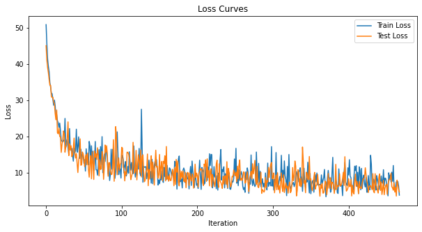
损失曲线是有噪声的,因为损失是在每次迭代时跟踪的,而不是多次迭代的平均值。
8.2 测试集的准确率
该函数对所有迷你批进行迭代,以获得测试集中全部 10,000 个样本的准确度。
total = 0
correct = 0

# drop_last switched to False to keep all samples
test_loader = DataLoader(mnist_test, batch_size=batch_size, shuffle=True, drop_last=False)

with torch.no_grad():
  net.eval()
  for data, targets in test_loader:
    data = data.to(device)
    targets = targets.to(device)

    # forward pass
    test_spk, _ = net(data.view(data.size(0), -1))

    # calculate total accuracy
    _, predicted = test_spk.sum(dim=0).max(1)
    total += targets.size(0)
    correct += (predicted == targets).sum().item()
>>> print(f"Total correctly classified test set images: {correct}/{total}")
>>> print(f"Test Set Accuracy: {100 * correct / total:.2f}%")
Total correctly classified test set images: 9387/10000
Test Set Accuracy: 93.87%
Voila!这就是要为静态 MNIST所做的全部。 你可以随意调整网络参数、超参数、衰减率、使用学习率调度程序等,看看能否提高网络性能。
结论
现在,你知道如何构建和训练一个静态数据集上的全连接网络。
脉冲神经元也可以适应其他层类型,包括卷积和跳跃连接。
掌握了这些知识,你现在应该能够构建许多不同类型的SNNs。
在 下一个教程 中,
你将学习如何训练脉冲卷积网络,并简化所需的代码量,使用 snn.backprop 模块。
此外,特别感谢 Bugra Kaytanli 为本教程提供了宝贵的反馈。
如果你喜欢这个项目,请考虑在 GitHub 上给代码仓库点亮星星⭐, 因为这是支持它的最简单的、最好的方式。