.. container:: cell markdown
` `__
.. rubric:: snnTorch - Spiking Autoencoder (SAE) using Convolutional
Spiking Neural Networks
:name: snntorch---spiking-autoencoder-sae-using-convolutional-spiking-neural-networks
.. rubric:: Tutorial by Alon Loeffler (www.alonloeffler.com)
:name: tutorial-by-alon-loeffler-wwwalonloefflercom
\*This tutorial is adapted from my original article published on
Medium.com
` `__
` `__
.. container:: cell markdown
For a comprehensive overview on how SNNs work, and what is going on
under the hood, `then you might be interested in the snnTorch
tutorial series available
here. `__
The snnTorch tutorial series is based on the following paper. If you
find these resources or code useful in your work, please consider
citing the following source:
`Jason K. Eshraghian, Max Ward, Emre Neftci, Xinxin Wang, Gregor Lenz, Girish
Dwivedi, Mohammed Bennamoun, Doo Seok Jeong, and Wei D. Lu. “Training
Spiking Neural Networks Using Lessons From Deep Learning”. Proceedings of the IEEE, 111(9) September 2023. `_
.. container:: cell markdown
In this tutorial, you will learn how to use snnTorch to:
- Create a spiking Autoencoder
- Reconstruct MNIST images
If running in Google Colab:
- You may connect to GPU by checking ``Runtime`` >
``Change runtime type`` > ``Hardware accelerator: GPU``
.. container:: cell markdown
.. rubric:: 1. Autoencoders
:name: 1-autoencoders
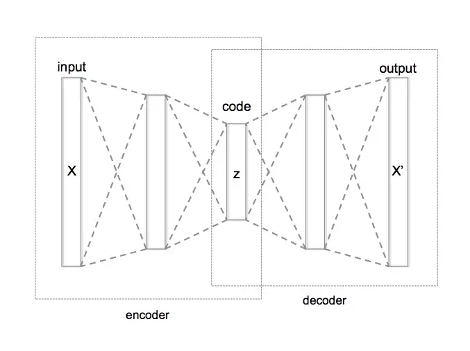
| An autoencoder is a neural network that is trained to reconstruct
its input data. It consists of two main components: 1) An encoder
| 2) A decoder
The encoder takes in input data (e.g. an image) and maps it to a
lower-dimensional latent space. For example an encoder might take in
as input a 28 x 28 pixel MNIST image (784 pixels total), and extract
the important features from the image while compressing it to a
smaller dimensionality (e.g. 32 features). This compressed
representation of the image is called the *latent representation*.
The decoder maps the latent representation back to the original input
space (i.e. from 32 features back to 784 pixels), and tries to
reconstruct the original image from a small number of key features.
.. raw:: html
Example of a simple Autoencoder where x is the input data, z is the encoded latent space, and x' is the reconstructed inputs once z is decoded (source: Wikipedia).
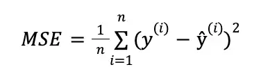
The goal of the autoencoder is to minimize the reconstruction error
between the input data and the output of the decoder.
This is achieved by training the model to minimize the reconstruction
loss, which is typically defined as the mean squared error (MSE)
between the input and the reconstructed output.
.. raw:: html
MSE loss equation. Here, $y$ would represent the original image (y true) and $\hat{y}$ would represent the reconstructed outputs (y pred) (source: Towards Data Science).
Autoencoders are excellent tools for reducing noise in data by
finding only the important parts of the data, and discarding
everything else during the reconstruction process. This is
effectively a dimensionality reduction tool.
.. container:: cell markdown
In this tutorial (similar to tutorial 1), we will assume we have some
non-spiking input data (i.e., the MNIST dataset) and that we want to
encode it and reconstruct it. So let's get started!
.. container:: cell markdown
.. rubric:: 2. Setting Up
:name: 2-setting-up
.. container:: cell markdown
.. rubric:: 2.1 Install/Import packages and set up environment
:name: 21-installimport-packages-and-set-up-environment
.. container:: cell markdown
To start, we need to install snnTorch and its dependencies (note this
tutorial assumes you have pytorch and torchvision already installed -
these come preinstalled in Colab). You can do this by running the
following command:
.. container:: cell code
.. code:: python
!pip install snntorch
.. container:: cell markdown
Next, let’s import the necessary modules and set up the SAE model.
We can use pyTorch to define the encoder and decoder networks, and
snnTorch to convert the neurons in the networks into leaky integrate
and fire (LIF) neurons, which read in and output spikes.
We will be using convolutional neural networks (CNN), covered in
tutorial 6, for the basis of our encoder and decoder.
.. container:: cell code
.. code:: python
import os
import torch
import torch.nn as nn
import torch.nn.functional as F
from torchvision import datasets, transforms
from torch.utils.data import DataLoader
from torchvision import utils as utls
import snntorch as snn
from snntorch import utils
from snntorch import surrogate
import numpy as np
#Define the SAE model:
class SAE(nn.Module):
def __init__(self,latent_dim):
super().__init__()
self.latent_dim = latent_dim #dimensions of the encoded z-space data
.. container:: cell markdown
.. rubric:: 3. Building the Autoencoder
:name: 3-building-the-autoencoder
.. container:: cell markdown
.. rubric:: 3.1 DataLoaders
:name: 31-dataloaders
We will be using the MNIST dataset
.. container:: cell code
.. code:: python
# dataloader arguments
batch_size = 250
data_path='/tmp/data/mnist'
dtype = torch.float
device = torch.device("cuda") if torch.cuda.is_available() else torch.device("mps") if torch.backends.mps.is_available() else torch.device("cpu")
.. container:: cell code
.. code:: python
# Define a transform
input_size = 32 #for the sake of this tutorial, we will be resizing the original MNIST from 28 to 32
transform = transforms.Compose([
transforms.Resize((input_size, input_size)),
transforms.Grayscale(),
transforms.ToTensor(),
transforms.Normalize((0,), (1,))])
# Load MNIST
# Training data
train_dataset = datasets.MNIST(root='dataset/', train=True, transform=transform, download=True)
train_loader = DataLoader(train_dataset, batch_size=batch_size, shuffle=True)
# Testing data
test_dataset = datasets.MNIST(root='dataset/', train=False, transform=transform, download=True)
test_loader = DataLoader(test_dataset, batch_size=batch_size, shuffle=True)
.. container:: cell markdown
.. rubric:: 3.2 The Encoder
:name: 32-the-encoder
Let's start building the sections of our autoencoder which we slowly
combine together to the SAE model we defined above:
.. container:: cell markdown
First, let's add an encoder with three convolutional layers
(``nn.Conv2d``), and one fully-connected linear output layer.
- We will use a kernel of size 3, with padding of 1 and stride of 2
for the CNN hyperparameters.
- We also add a Batch Norm layer between convolutional layers. Since
will be using the neuron membrane potential as outputs from each
neuron, normalization will help our training process.
.. container:: cell code
.. code:: python
#Define the SAE model:
class SAE(nn.Module):
def __init__(self):
super().__init__()
self.latent_dim = latent_dim #dimensions of the encoded z-space data
# Encoder
self.encoder = nn.Sequential(nn.Conv2d(1, 32, 3,padding = 1,stride=2), # Conv Layer 1
nn.BatchNorm2d(32),
snn.Leaky(beta=beta, spike_grad=spike_grad, init_hidden=True,threshold=thresh), #SNN TORCH LIF NEURON
nn.Conv2d(32, 64, 3,padding = 1,stride=2), # Conv Layer 2
nn.BatchNorm2d(64),
snn.Leaky(beta=beta, spike_grad=spike_grad, init_hidden=True,threshold=thresh),
nn.Conv2d(64, 128, 3,padding = 1,stride=2), # Conv Layer 3
nn.BatchNorm2d(128),
snn.Leaky(beta=beta, spike_grad=spike_grad, init_hidden=True,threshold=thresh),
nn.Flatten(start_dim = 1, end_dim = 3), #Flatten convolutional output
nn.Linear(128*4*4, latent_dim), # Fully connected linear layer
snn.Leaky(beta=beta, spike_grad=spike_grad, init_hidden=True, output=True,threshold=thresh)
)
.. container:: cell markdown
.. rubric:: 3.3 The Decoder
:name: 33-the-decoder
.. container:: cell markdown
Before we write the decoder, there is one more small step required.
When decoding the latent z-space data, we need to move from the
flattened encoded representation (latent_dim) back to a tensor
representation to use in transposed convolution.
To do so, we need to run an additional fully-connected linear layer
transforming the data back into a tensor of 128 x 4 x 4.
.. container:: cell code
.. code:: python
#Define the SAE model:
class SAE(nn.Module):
def __init__(self,latent_dim):
super().__init__()
self.latent_dim = latent_dim #dimensions of the encoded z-space data
# Encoder
self.encoder = nn.Sequential(nn.Conv2d(1, 32, 3,padding = 1,stride=2), # Conv Layer 1
nn.BatchNorm2d(32),
snn.Leaky(beta=beta, spike_grad=spike_grad, init_hidden=True,threshold=thresh), #SNN TORCH LIF NEURON
nn.Conv2d(32, 64, 3,padding = 1,stride=2), # Conv Layer 2
nn.BatchNorm2d(64),
snn.Leaky(beta=beta, spike_grad=spike_grad, init_hidden=True,threshold=thresh),
nn.Conv2d(64, 128, 3,padding = 1,stride=2), # Conv Layer 3
nn.BatchNorm2d(128),
snn.Leaky(beta=beta, spike_grad=spike_grad, init_hidden=True,threshold=thresh),
nn.Flatten(start_dim = 1, end_dim = 3), #Flatten convolutional output
nn.Linear(128*4*4, latent_dim), # Fully connected linear layer
snn.Leaky(beta=beta, spike_grad=spike_grad, init_hidden=True, output=True,threshold=thresh)
)
# From latent back to tensor for convolution
self.linearNet= nn.Sequential(nn.Linear(latent_dim,128*4*4),
snn.Leaky(beta=beta, spike_grad=spike_grad, init_hidden=True, output=True,threshold=thresh))
.. container:: cell markdown
Now we can write the decoder, with three transposed convolutional
(``nn.ConvTranspose2d``) layers and one linear output layer. Although
we converted the latent data back into tensor form for convolution,
we still need to Unflatten it to a tensor of 128 x 4 x 4, as the
input to the network is 1 dimensional. This is done using
``nn.Unflatten`` in the first line of the Decoder.
.. container:: cell code
.. code:: python
#Define the SAE model:
class SAE(nn.Module):
def __init__(self,latent_dim):
super().__init__()
self.latent_dim = latent_dim #dimensions of the encoded z-space data
# Encoder
self.encoder = nn.Sequential(nn.Conv2d(1, 32, 3,padding = 1,stride=2), # Conv Layer 1
nn.BatchNorm2d(32),
snn.Leaky(beta=beta, spike_grad=spike_grad, init_hidden=True,threshold=thresh), #SNN TORCH LIF NEURON
nn.Conv2d(32, 64, 3,padding = 1,stride=2), # Conv Layer 2
nn.BatchNorm2d(64),
snn.Leaky(beta=beta, spike_grad=spike_grad, init_hidden=True,threshold=thresh),
nn.Conv2d(64, 128, 3,padding = 1,stride=2), # Conv Layer 3
nn.BatchNorm2d(128),
snn.Leaky(beta=beta, spike_grad=spike_grad, init_hidden=True,threshold=thresh),
nn.Flatten(start_dim = 1, end_dim = 3), #Flatten convolutional output
nn.Linear(128*4*4, latent_dim), # Fully connected linear layer
snn.Leaky(beta=beta, spike_grad=spike_grad, init_hidden=True, output=True,threshold=thresh)
)
# From latent back to tensor for convolution
self.linearNet = nn.Sequential(nn.Linear(latent_dim,128*4*4),
snn.Leaky(beta=beta, spike_grad=spike_grad, init_hidden=True, output=True,threshold=thresh))
# Decoder
self.decoder = nn.Sequential(nn.Unflatten(1,(128,4,4)), #Unflatten data from 1 dim to tensor of 128 x 4 x 4
snn.Leaky(beta=beta, spike_grad=spike_grad, init_hidden=True,threshold=thresh),
nn.ConvTranspose2d(128, 64, 3,padding = 1,stride=(2,2),output_padding=1),
nn.BatchNorm2d(64),
snn.Leaky(beta=beta, spike_grad=spike_grad, init_hidden=True,threshold=thresh),
nn.ConvTranspose2d(64, 32, 3,padding = 1,stride=(2,2),output_padding=1),
nn.BatchNorm2d(32),
snn.Leaky(beta=beta, spike_grad=spike_grad, init_hidden=True,threshold=thresh),
nn.ConvTranspose2d(32, 1, 3,padding = 1,stride=(2,2),output_padding=1),
snn.Leaky(beta=beta, spike_grad=spike_grad, init_hidden=True,output=True,threshold=20000) #make large so membrane can be trained
)
.. container:: cell markdown
One important thing to note is in the final Leaky layer, our spiking
threshold (``thresh``) is set extremely high. This is a neat trick in
snnTorch, which allows the neuron membrane in the final layer to
continuously be updated, without ever reaching a spiking threshold.
The output of each Leaky Neuron will consist of a tensor of spikes (0
or 1) and a tensor of neuron membrane potential (negative or positive
real numbers). snnTorch allows us to use either the spikes or
membrane potential of each neuron in training. We will be using the
membrane potential output from the final layer for the image
reconstruction.
.. container:: cell markdown
.. rubric:: 3.4 Forward Function
:name: 34-forward-function
Finally, let’s write the forward, encode and decode functions, before
putting it all together
.. container:: cell code
.. code:: python
def forward(self, x):
utils.reset(self.encoder) #need to reset the hidden states of LIF
utils.reset(self.decoder)
utils.reset(self.linearNet)
#encode
spk_mem=[];spk_rec=[];encoded_x=[]
for step in range(num_steps): #for t in time
spk_x,mem_x=self.encode(x) #Output spike trains and neuron membrane states
spk_rec.append(spk_x)
spk_mem.append(mem_x)
spk_rec=torch.stack(spk_rec,dim=2) # stack spikes in second tensor dimension
spk_mem=torch.stack(spk_mem,dim=2) # stack membranes in second tensor dimension
#decode
spk_mem2=[];spk_rec2=[];decoded_x=[]
for step in range(num_steps): #for t in time
x_recon,x_mem_recon=self.decode(spk_rec[...,step])
spk_rec2.append(x_recon)
spk_mem2.append(x_mem_recon)
spk_rec2=torch.stack(spk_rec2,dim=4)
spk_mem2=torch.stack(spk_mem2,dim=4)
out = spk_mem2[:,:,:,:,-1] #return the membrane potential of the output neuron at t = -1 (last t)
return out
def encode(self,x):
spk_latent_x,mem_latent_x=self.encoder(x)
return spk_latent_x,mem_latent_x
def decode(self,x):
spk_x,mem_x = self.latentToConv(x) #convert latent dimension back to total size of features in encoder final layer
spk_x2,mem_x2=self.decoder(spk_x)
return spk_x2,mem_x2
.. container:: cell markdown
There are a couple of key things to notice here:
1) At the beginning of each call of our forward function, we need to
reset the hidden weights of each LIF neuron. If we do not do this, we
will get weird gradient errors from pytorch when we try to backprop.
To do so we use ``utils.reset``.
2) In the forward function, when we call the encode and decode
functions, we do so in a loop. This is because we are converting
static images into spike trains, as explained previously. Spike
trains need a time, t, during which spiking can occur or not occur.
Therefore, we encode and decode the original image :math:`t` (or
``num_steps``) times, to create a latent representation, :math:`z`.
.. container:: cell markdown
For example, converting a sample digit 7 from the MNIST dataset into
a spike-train with a latent dimension of 32 and t = 50, might look
like this: Spike-Train of sample MNIST digit 7 after encoding. Other
instances of 7 will have slightly different spike-trains, and
different digits will have even more different spike-trains.
.. container:: cell markdown
.. rubric:: 3.5 Putting it all together:
:name: 35-putting-it-all-together
Our final, complete SAE class should look like this:
.. container:: cell code
.. code:: python
class SAE(nn.Module):
def __init__(self):
super().__init__()
#Encoder
self.encoder = nn.Sequential(nn.Conv2d(1, 32, 3,padding = 1,stride=2),
nn.BatchNorm2d(32),
snn.Leaky(beta=beta, spike_grad=spike_grad, init_hidden=True,threshold=thresh),
nn.Conv2d(32, 64, 3,padding = 1,stride=2),
nn.BatchNorm2d(64),
snn.Leaky(beta=beta, spike_grad=spike_grad, init_hidden=True,threshold=thresh),
nn.Conv2d(64, 128, 3,padding = 1,stride=2),
nn.BatchNorm2d(128),
snn.Leaky(beta=beta, spike_grad=spike_grad, init_hidden=True,threshold=thresh),
nn.Flatten(start_dim = 1, end_dim = 3),
nn.Linear(2048, latent_dim), #this needs to be the final layer output size (channels * pixels * pixels)
snn.Leaky(beta=beta, spike_grad=spike_grad, init_hidden=True, output=True,threshold=thresh)
)
# From latent back to tensor for convolution
self.linearNet= nn.Sequential(nn.Linear(latent_dim,128*4*4),
snn.Leaky(beta=beta, spike_grad=spike_grad, init_hidden=True, output=True,threshold=thresh)) #Decoder
self.decoder = nn.Sequential(nn.Unflatten(1,(128,4,4)),
snn.Leaky(beta=beta, spike_grad=spike_grad, init_hidden=True,threshold=thresh),
nn.ConvTranspose2d(128, 64, 3,padding = 1,stride=(2,2),output_padding=1),
nn.BatchNorm2d(64),
snn.Leaky(beta=beta, spike_grad=spike_grad, init_hidden=True,threshold=thresh),
nn.ConvTranspose2d(64, 32, 3,padding = 1,stride=(2,2),output_padding=1),
nn.BatchNorm2d(32),
snn.Leaky(beta=beta, spike_grad=spike_grad, init_hidden=True,threshold=thresh),
nn.ConvTranspose2d(32, 1, 3,padding = 1,stride=(2,2),output_padding=1),
snn.Leaky(beta=beta, spike_grad=spike_grad, init_hidden=True,output=True,threshold=20000) #make large so membrane can be trained
)
def forward(self, x): #Dimensions: [Batch,Channels,Width,Length]
utils.reset(self.encoder) #need to reset the hidden states of LIF
utils.reset(self.decoder)
utils.reset(self.linearNet)
#encode
spk_mem=[];spk_rec=[];encoded_x=[]
for step in range(num_steps): #for t in time
spk_x,mem_x=self.encode(x) #Output spike trains and neuron membrane states
spk_rec.append(spk_x)
spk_mem.append(mem_x)
spk_rec=torch.stack(spk_rec,dim=2)
spk_mem=torch.stack(spk_mem,dim=2) #Dimensions:[Batch,Channels,Width,Length, Time]
#decode
spk_mem2=[];spk_rec2=[];decoded_x=[]
for step in range(num_steps): #for t in time
x_recon,x_mem_recon=self.decode(spk_rec[...,step])
spk_rec2.append(x_recon)
spk_mem2.append(x_mem_recon)
spk_rec2=torch.stack(spk_rec2,dim=4)
spk_mem2=torch.stack(spk_mem2,dim=4)#Dimensions:[Batch,Channels,Width,Length, Time]
out = spk_mem2[:,:,:,:,-1] #return the membrane potential of the output neuron at t = -1 (last t)
return out #Dimensions:[Batch,Channels,Width,Length]
def encode(self,x):
spk_latent_x,mem_latent_x=self.encoder(x)
return spk_latent_x,mem_latent_x
def decode(self,x):
spk_x,mem_x = self.linearNet(x) #convert latent dimension back to total size of features in encoder final layer
spk_x2,mem_x2=self.decoder(spk_x)
return spk_x2,mem_x2
.. container:: cell markdown
.. rubric:: 4. Training and Testing
:name: 4-training-and-testing
Finally, we can move on to training our SAE, and testing its
usefulness. We have already loaded the MNIST dataset, and split it
into training and testing classes.
.. container:: cell markdown
.. rubric:: 4.1 Training Function
:name: 41-training-function
We define our training function, which takes in the network model,
training dataset, optimizer and epoch number as inputs, and returns
the loss value after running all batches of the current epoch.
As discussed at the beginning, we will be using MSE loss to compare
the reconstructed image (``x_recon``) with the original image
(``real_img``)
As always, to set up our gradients for backprop we use
``opti.zero_grad()``, and then call ``loss_val.backward()`` and
``opti.step()`` to perform backprop.
.. container:: cell code
.. code:: python
#Training
def train(network, trainloader, opti, epoch):
network=network.train()
train_loss_hist=[]
for batch_idx, (real_img, labels) in enumerate(trainloader):
opti.zero_grad()
real_img = real_img.to(device)
labels = labels.to(device)
#Pass data into network, and return reconstructed image from Membrane Potential at t = -1
x_recon = network(real_img) #Dimensions passed in: [Batch_size,Input_size,Image_Width,Image_Length]
#Calculate loss
loss_val = F.mse_loss(x_recon, real_img)
print(f'Train[{epoch}/{max_epoch}][{batch_idx}/{len(trainloader)}] Loss: {loss_val.item()}')
loss_val.backward()
opti.step()
#Save reconstructed images every at the end of the epoch
if batch_idx == len(trainloader)-1:
# NOTE: you need to create training/ and testing/ folders in your chosen path
utls.save_image((real_img+1)/2, f'figures/training/epoch{epoch}_finalbatch_inputs.png')
utls.save_image((x_recon+1)/2, f'figures/training/epoch{epoch}_finalbatch_recon.png')
return loss_val
.. container:: cell markdown
.. rubric:: 4.2 Testing Function
:name: 42-testing-function
The testing function is nearly identifcal to the training function,
except we do not backpropagate, therefore no gradients are required
and we use ``torch.no_grad()``
.. container:: cell code
.. code:: python
#Testing
def test(network, testloader, opti, epoch):
network=network.eval()
test_loss_hist=[]
with torch.no_grad(): #no gradient this time
for batch_idx, (real_img, labels) in enumerate(testloader):
real_img = real_img.to(device)#
labels = labels.to(device)
x_recon = network(real_img)
loss_val = F.mse_loss(x_recon, real_img)
print(f'Test[{epoch}/{max_epoch}][{batch_idx}/{len(testloader)}] Loss: {loss_val.item()}')#, RECONS: {recons_meter.avg}, DISTANCE: {dist_meter.avg}')
if batch_idx == len(testloader)-1:
utls.save_image((real_img+1)/2, f'figures/testing/epoch{epoch}_finalbatch_inputs.png')
utls.save_image((x_recon+1)/2, f'figures/testing/epoch{epoch}_finalbatch_recons.png')
return loss_val
.. container:: cell markdown
There are a couple of ways to calculate loss with spiking neural
networks. Here, we are simply taking the membrane potential of the
final fully-connected layer of neurons at the last time step
(:math:`t = 5`).
Therefore, we only need to compare each original image with its
corresponding decoded, reconstructed image once per epoch. We can
also return the membrane potentials at each time step, and create t
different versions of the reconstructed image, and then compare each
of them with the original image and take the average loss. For those
of you interested in this, you can replace the loss function above
with something like this:
(*note this will fail to run as we have not defined any of the
variables yet, it is just here for illustrative purposes*)
.. container:: cell code
.. code:: python
train_loss_hist=[]
loss_val = torch.zeros((1), dtype=dtype, device=device)
for step in range(num_steps):
loss_val += F.mse_loss(x_recon, real_img)
train_loss_hist.append(loss_val.item())
avg_loss=loss_val/num_steps
.. container:: output error
::
---------------------------------------------------------------------------
NameError Traceback (most recent call last)
Cell In[72], line 4
2 loss_val = torch.zeros((1), dtype=dtype, device=device)
3 for step in range(num_steps):
----> 4 loss_val += F.mse_loss(x_recon, real_img)
5 train_loss_hist.append(loss_val.item())
6 avg_loss=loss_val/num_steps
NameError: name 'x_recon' is not defined
.. container:: cell markdown
.. rubric:: 5. Conclusion: Running the SAE
:name: 5-conclusion-running-the-sae
Now, finally, we can run our SAE model. Let’s define some parameters,
and run training and testing
.. container:: cell markdown
Let's create directories where we can save our original and
reconstructed images for training and testing:
.. container:: cell code
.. code:: python
# create training/ and testing/ folders in your chosen path
if not os.path.isdir('figures/training'):
os.makedirs('figures/training')
if not os.path.isdir('figures/testing'):
os.makedirs('figures/testing')
.. container:: cell code
.. code:: python
# dataloader arguments
batch_size = 250
input_size = 32 #resize of mnist data (optional)
#setup GPU
dtype = torch.float
device = torch.device("cuda") if torch.cuda.is_available() else torch.device("cpu")
# neuron and simulation parameters
spike_grad = surrogate.atan(alpha=2.0)# alternate surrogate gradient fast_sigmoid(slope=25)
beta = 0.5 #decay rate of neurons
num_steps=5
latent_dim = 32 #dimension of latent layer (how compressed we want the information)
thresh=1#spiking threshold (lower = more spikes are let through)
epochs=10
max_epoch=epochs
#Define Network and optimizer
net=SAE()
net = net.to(device)
optimizer = torch.optim.AdamW(net.parameters(),
lr=0.0001,
betas=(0.9, 0.999),
weight_decay=0.001)
#Run training and testing
for e in range(epochs):
train_loss = train(net, train_loader, optimizer, e)
test_loss = test(net,test_loader,optimizer,e)
.. container:: output stream stdout
::
Train[0/10][0/240] Loss: 0.10109379142522812
Train[0/10][1/240] Loss: 0.10465191304683685
.. container:: output stream stderr
::
KeyboardInterrupt
.. container:: cell markdown
After only 10 epochs, our training and testing reconstructed losses
should be around 0.05, and our reconstructed images should look
something like this:
.. container:: cell markdown
.. container:: cell markdown
Yes, the reconstructed images are a bit blurry, and the loss isn’t
perfect, but from only 10 epochs, and only using the final membrane
potential at :math:`t = 5` for our reconstructed loss, it’s a pretty
decent start!
.. container:: cell markdown
Try increasing the number of epochs, or playing around with
``thresh``, ``num_steps`` and ``batch_size`` to see if you can get
better loss!